Old Houses, New Profits?

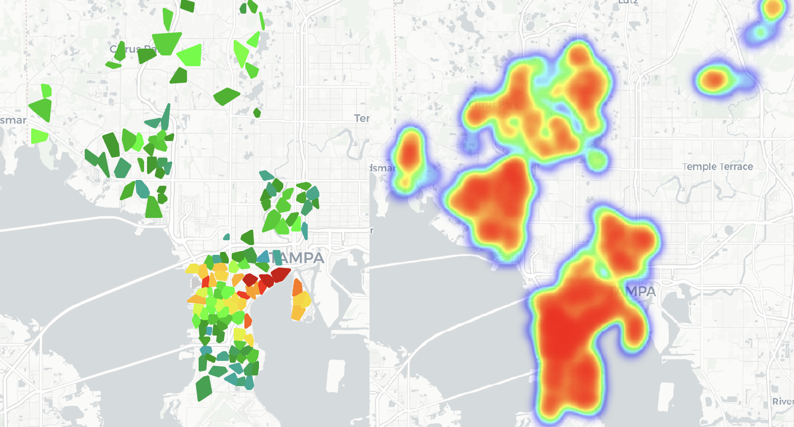
Map highlighting top opportunities in Tampa.

The Motivation

I’m helping organize BRASA Connect 2025, a student-led conference at my university. A rewarding part of this work is inviting professionals with impressive careers to share their experiences with students who are just beginning theirs.

At one meeting to select speakers and mentors, I met someone involved in startups. He described how a real estate development fund operates in Florida, and that caught my interest.

The U.S. real estate market is varied, but some neighborhoods consistently withstand economic downturns better than others. Why? These areas have strong fundamentals: good schools, solid local economies, and high household incomes.

Many of these neighborhoods are also old. The average house is 43 years old, with some over 70. At a certain point, renovating these homes stops making financial sense. Add to that the trend of people moving from struggling states to the fast-growing Sun Belt, especially Florida and Texas, and it’s clear why demand for housing in these areas keeps rising.

Here’s the interesting part: on the same street, you might see a 1950s house worth X, while a new house on the same lot is worth nearly 3X.

The fund’s strategy is simple: buy old houses in established neighborhoods, demolish them, and build new ones.

But does this really work? It sounds promising—maybe too promising. In a world where tech companies have sky-high valuations, a real estate fund offering nearly 20% annual returns in dollars seems too good to pass up.

I wanted to know if the numbers backed up the story. I’d never done a data science project focused on price forecasting before, so this was the perfect chance to learn. And there’s no shortage of real estate data. All I needed to do was collect it, analyze it, and see if the results matched the theory.

Data Collection

Finding the data was straightforward. I started by looking for ready-made datasets on Kaggle, but nothing was specific enough to Florida or the cities I was interested in. The closest I found was a dataset with over 100,000 rows covering the whole U.S., but it was too broad to be useful. Still, it pointed me in the right direction: Realtor.com.

Realtor.com, like Zillow, lists homes for sale, rent, and recently sold properties, all pulled from MLS (Multiple Listing Services). The key difference? It’s much easier to scrape data from Realtor.com than Zillow. A quick search for "Realtor web scraping" showed plenty of paid options, but I found a free GitHub repository that fit my needs: HomeHarvest.

With this tool, I could pull detailed CSV files with everything from addresses and sale prices to square footage, tax info, and even nearby schools. I could also filter by city and listing type—whether homes were for sale, rent, or recently sold—making data collection efficient and precise.

from homeharvest import scrape_property

properties = scrape_property(
  location="San Diego, CA",
  listing_type="sold",  # options: for_sale, for_rent, pending
  past_days=30,  # sold in the last 30 days; for_sale/for_rent means listed in the last 30 days
)

print(properties.head())

Output:

>>> properties.head()
    MLS       MLS # Status          Style  ...     COEDate LotSFApx PrcSqft Stories
0  SDCA   230018348   SOLD         CONDOS  ...  2023-10-03   290110     803       2
1  SDCA   230016614   SOLD      TOWNHOMES  ...  2023-10-03     None     838       3
2  SDCA   230016367   SOLD         CONDOS  ...  2023-10-03    30056     649       1
3  MRCA  NDP2306335   SOLD  SINGLE_FAMILY  ...  2023-10-03     7519     661       2
4  SDCA   230014532   SOLD         CONDOS  ...  2023-10-03     None     752       1
[5 rows x 22 columns]

But there was a limitation. HomeHarvest capped each query at 10,000 listings. I tried adjusting the code, but it seemed this limit was set by Realtor.com’s servers.

To work around this, I wrote a script that pulled listings month by month for each city over the past five years. Breaking the data into smaller chunks kept me under the limit. I also added random pauses between requests to avoid errors from sending too many queries at once.

In under two hours, I had collected 192,706 sold property listings from Tampa, Orlando, Winter Garden, and Winter Park, complete with detailed information from the last five years.

Data Cleaning

It had been a while since I worked with data. The last time was during an internship at Stone Pagamentos in Brazil, where I analyzed financial data for the commercial team. Even then, I didn’t go deep into predictive analysis.

After cleaning the dataset, I realized a lot of the data wasn’t usable. Out of 192,706 records, I had to remove:

60,000 that weren’t single-family homes
10,000 with too many missing values
10,000 duplicates

I also needed to handle outliers to avoid skewing the analysis. Some properties were listed at prices like $0,$ 1, or $9,999,999. Others had unrealistically large sizes, like 9999 square feet. To make sure the dataset reflected real market conditions, I filtered out these anomalies:

df = df[
    (df['estimated_value'] > 100000) &  # Removing unrealistically low prices
    (df['estimated_value'] < 5000000) &  # Excluding overly high valuations
    (df['year_built'] >= 1901) &  # Filtering out properties with impossible construction years
    (df['sqft'] <= 5000)  # Eliminating properties with unrealistic square footage
]

After this, I was left with just over 109,000 clean property listings.

To add more depth to the analysis, I incorporated median income data by ZIP Code. This gave valuable context, helping me see how property prices related to the economic conditions in each area.